This is the third and final part of my series of tutorials showing how I created a model of the Earth. If you missed part one, I showed you how to create the simple model and add the basic color/bump image maps. In part two, I showed you how to add shader layers for the ocean, clouds, and the night city lights.
Because LightWave does not have volumetric shading support, we are going to fake an atmosphere glow using a flat, transparent object. Using the node editor, we will control the transparency based on its relation to the light vector.
Setup the Atmosphere Disk
- Enable the “Earth:Atmosphere” object in the Scene editor and select the object in the scene.
- Edit the motion properties for the object (‘m’). Set the “Target Item” to the camera. Now, the atmosphere disc will always appear to be surrounding the earth when viewed through that camera.
Add Basic Textures to the Atmosphere Disk
- Open the Surface Editor and select the Atmosphere surface. Change the Color to 56, 130, 255. Set Luminosity to 100% and Diffuse to 0%. Make sure “Smoothing” is enabled.
- Back on the Basic tab, enable nodes and launch the Node Editor.
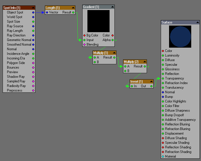
- We will now create a radial gradient from the center of the atmosphere disk. Create a “Spot Info” node (Spot->Spot Info) and a vector Length node (Math->Vector->Length). Connect the “Object Spot” output from “Spot Info” to the “Vector” input of Length.
- Create a “Gradient’ node (Gradient->Gradient). Connect the “Result” output from “Length” to the Input node of Gradient. Add the following keys to the Gradient node:
- Position: 1.0, Color: (0, 0, 0), Alpha: 33%
- Position: 1.14, Color: (0, 0, 0), Alpha: 0%
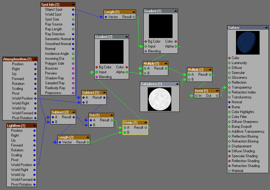
- Next, create the nodes that will end up connecting to the “Transparency” of the surface. Create 2 “Multiply” nodes (Math->Scalar->Multiply) and one Invert node (Math->Scalar->Invert).
- Connect the “Alpha” output from Gradient to the “A” input of “Multiply (1)”. Connect the “Result” output from “Multiply (1)” to the “A” input of “Multiply (2)”. Connect the “Result” output of “Multiply (2)” to the “In” value of Invert. And connect the “Out” of Invert to the “Transparency” input of the Surface node.
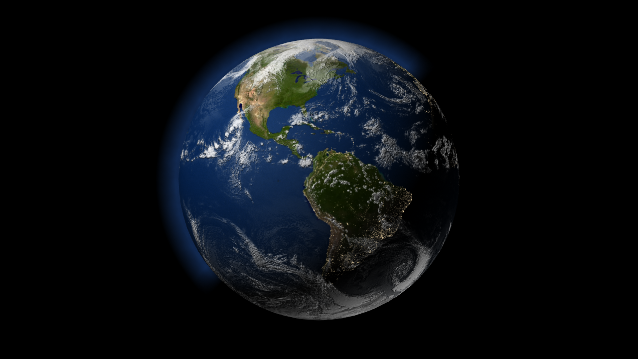
- If you set the “B” values manually in the “Multiply” nodes and render, you will see a blue atmosphere completely surrounding the earth.
Link the Atmospheric Glow to the Light Source
- Add a turbulence node (3D Textures->Turbulence). Set the “BG Color” to 218, 218, 218. Set the “FG Color” to 255, 255, 255. Set the Scale X, Y, Z to 10cm, 10cm, 10cm.
- Connect the “Color” output from Turbulence to the “B” input of “Multiply (2)”.
- Add an Item Info node (Item Info->Item Info). Rename it to “AtmosphereItem”. Set the item to reference the Earth:Atmosphere object.
- Create another Item Info node and rename it to “LightItem”. Set the item to reference your scene light.
- Create a new vector Subtract node (Math->Vector->Subtract). Connect the “World Spot” output of “Spot Info” to the “A” input of Subtract. Connect the “World Position” output of “AtmosphereItem” to the “B” input of Subtract. The output of the Subtract node is a vector that represents the ray from the center of the atmosphere disk to the evaluated point.
- Create another vector Subtract node. Connect the “World Position” of “LightItem” to “A” and the “World Position” of “AtmosphereItem” to “B”. The output of this Subtract node is the vector pointing from the center of the Atmosphere object to the light.
- Create a “Dot” node (Math->Vector->Dot). Connect the output of the first Subtract node to “A” and the output of the second Subtract node to “B”. The output of the Dot node is a scalar value representing how strong the light is hitting the surface (the light angle).
- Create a vector Length node (Math->Vector->Length) and a scalar Divide node (Math->Scalar->Divide). Connect the output of the Dot node to the “A” input of Divide. Connect the output of the second Subtract node to the input of the Length node, and then connect that output to the “B” input of the Divide. Now the Divide output represents a normalized value of the light angle.
- Create a gradient node. Connect the Divide output to the “Input” value of the gradient. Add these keys:
- Position: -0.0242, Alpha: 0%
- Position: 0.1004, Alpha 100%
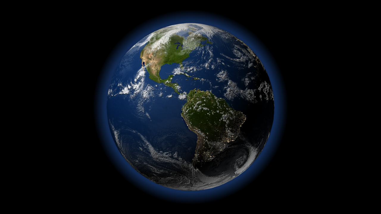
- Finally, connect the output of the gradient to the “B” input of “Multiply (1)”. Run a test render to see the result.